概述
一个点的接近中心性(Closeness Centrality)是由该点到它可连通的其它各点的最短距离的平均值来衡量的。一个点与其他所有点相距越近,这个点的中心性就越高。接近中心性算法广泛应用于关键社交节点发现、功能性场所选址等场景。
接近中心性算法更适用于连通图。对于非连通图,推荐使用它的变体——调和中心性。
接近中心性的取值范围是0到1,节点的分值越大,距离其他节点越近。
接近中心性的原始概念是由Alex Bavelas于1950年提出的:
- A. Bavelas, Communication patterns in task-oriented groups (1950)
基本概念
最短距离
两个点之间的最短距离是指它们之间最短路径的边数。最短路径是按照BFS的原则进行寻找的,如果将一个点看作起点,另一个点是该点的第K步邻居,它们之间的最短距离就是K。关于BFS和K邻的详细介绍,请阅读全图K邻。
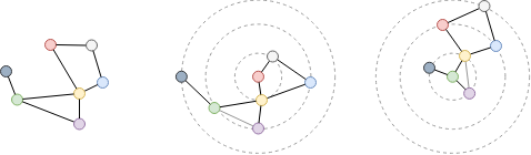
考察以上无向图中红、绿两点之间的最短距离。由于是无向图,无论是以红色还是绿色节点为起点,它们均为对方的2步邻居,即它们的最短距离为2。
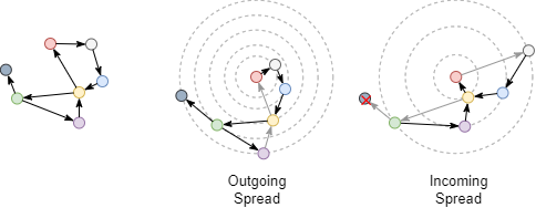
将上面的无向图修改为有向图后,再次考察红、绿两点之间的最短距离。如果考虑边的方向。从红色节点到绿色节点入方向最短距离为3,出方向最短距离为4。
当考虑边权重时,两个节点之间的最短距离是它们之间路径中边的最小权重之和。
在为边分配权重后,检查红色和绿色节点之间的最短距离。为了最小化总权重,选择具有更多边的路径,从而产生总权重5。

接近中心性
在本算法中,节点的接近中心性分值等于该点与其他能够相连的各节点的最短距离算数平均值(Arithmetic Mean)的倒数。计算公式为:
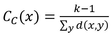
其中,x为待计算的目标节点,y为通过边与x相连的任意一个节点(不包含x),k-1为y的个数,d(x,y)为x到y的最短距离。
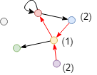
计算上图中红色节点入方向的接近中心性。入方向上红色节点仅可连通蓝、黄、紫三个节点,故其接近中心性为3 / (2 + 1 + 2) = 0.6。通过入边不可达的绿色、灰色节点不参与计算。
接近中心性算法会消耗很多计算资源。在一个有V个节点的图中,建议当V>10000时通过采样进行近似计算,推荐的采样个数是节点数以10为底的对数(
log(V))。
每次执行算法时,只进行一次采样,每个节点的中心性分值是基于该节点到所有样本节点的最短距离计算的。
特殊说明
- 孤点的接近中心性分值为0。
- 计算某点的接近中心性时,会排除那些不可连通的节点,比如孤点、其他连通分量内的点或是虽然属于同一连通分量但在规定的方向上不可达的节点等。
示例图
在一个空图中运行以下语句定义图结构并插入数据:
ALTER GRAPH CURRENT_GRAPH ADD NODE {
user ()
};
ALTER GRAPH CURRENT_GRAPH ADD EDGE {
vote ()-[{strength uint32}]->()
};
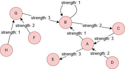
INSERT (A:user {_id: "A"}),
(B:user {_id: "B"}),
(C:user {_id: "C"}),
(D:user {_id: "D"}),
(E:user {_id: "E"}),
(F:user {_id: "F"}),
(G:user {_id: "G"}),
(H:user {_id: "H"}),
(A)-[:vote {strength: 1}]->(B),
(A)-[:vote {strength: 3}]->(E),
(B)-[:vote {strength: 1}]->(B),
(B)-[:vote {strength: 2}]->(C),
(C)-[:vote {strength: 3}]->(A),
(D)-[:vote {strength: 2}]->(A),
(F)-[:vote {strength: 2}]->(G),
(G)-[:vote {strength: 3}]->(B),
(H)-[:vote {strength: 1}]->(G);
create().node_schema("user").edge_schema("vote");
create().edge_property(@vote, "strength", uint32);
insert().into(@user).nodes([{_id:"A"},{_id:"B"},{_id:"C"},{_id:"D"},{_id:"E"},{_id:"F"},{_id:"G"},{_id:"H"}]);
insert().into(@vote).edges([{_from:"A", _to:"B", strength:1}, {_from:"A", _to:"E", strength:3}, {_from:"B", _to:"B", strength:1}, {_from:"B", _to:"C", strength:2}, {_from:"C", _to:"A", strength:3}, {_from:"D", _to:"A", strength:2}, {_from:"F", _to:"G", strength:2}, {_from:"G", _to:"B", strength:3}, {_from:"H", _to:"G", strength:1}]);
在HDC图上运行算法
创建HDC图
将当前图集全部加载到HDC服务器hdc-server-1上,并命名为 my_hdc_graph:
CREATE HDC GRAPH my_hdc_graph ON "hdc-server-1" OPTIONS {
  nodes: {"*": ["*"]},
  edges: {"*": ["*"]},
  direction: "undirected",
  load_id: true,
  update: "static"
}
hdc.graph.create("my_hdc_graph", {
  nodes: {"*": ["*"]},
  edges: {"*": ["*"]},
  direction: "undirected",
  load_id: true,
  update: "static"
}).to("hdc-server-1")
参数
算法名:closeness_centrality
参数名 |
类型 |
规范 |
默认值 |
可选 |
描述 |
|---|---|---|---|---|---|
ids |
[]_id |
/ | / | 是 | 通过_id指定参与计算的点;若未设置则计算所有点 |
uuids |
[]_uuid |
/ | / | 是 | 通过_uuid指定参与计算的点;若未设置则计算所有点 |
direction |
String | in, out |
/ | 是 | 指定最短路径中所有边的方向,in表示仅包含入边,out表示仅包含出边 |
edge_schema_property |
[]"<@schema.?><property>" |
/ | / | 是 | 作为权重的数值类型边属性,权重值为所有指定属性值的总和;不包含指定属性的边将被忽略 |
impl_type |
String | dijkstra, delta_stepping, spfa, beta |
beta |
是 | 指定计算加权最短路径的算法:Dijkstra、Delta-Stepping、SPFA或嬴图默认最短路径算法beta。仅当使用edge_schema_property时生效 |
sample_size |
Integer | -1, -2, [1, |V|] |
-2 |
是 | 指定采样策略:
|
return_id_uuid |
String | uuid, id, both |
uuid |
是 | 在结果中使用_uuid、_id或同时使用两者来表示点 |
limit |
Integer | ≥-1 | -1 |
是 | 限制返回的结果数;-1返回所有结果 |
order |
String | asc, desc |
/ | 是 | 根据closeness_centrality分值对结果排序 |
文件回写
CALL algo.closeness_centrality.write("my_hdc_graph", {
  return_id_uuid: "id"
}, {
  file: {
    filename: "closeness"
  }
})
algo(closeness_centrality).params({
  projection: "my_hdc_graph",
  return_id_uuid: "id"
}).write({
  file: {
    filename: "closeness"
  }
})
结果:
_id,closeness_centrality
G,0.538462
D,0.388889
F,0.368421
H,0.368421
B,0.636364
A,0.583333
E,0.388889
C,0.5
数据库回写
将结果中的closeness_centrality值写入指定点属性。该属性类型为float。
CALL algo.closeness_centrality.write("my_hdc_graph", {},
{
  db: {
    property: "cc"
  }
})
algo(closeness_centrality).params({
  projection: "my_hdc_graph"
}).write({
  db:{
    property: 'cc'
  }
})
完整返回
CALL algo.closeness_centrality.run("my_hdc_graph", {
  return_id_uuid: "id",
  ids: ["A", "B"],
  edge_schema_property: "strength"
}) YIELD cc
RETURN cc
exec{
  algo(closeness_centrality).params({
    return_id_uuid: "id",
    ids: ["A", "B"],
    edge_schema_property: "strength"
  }) as cc
  return cc
} on my_hdc_graph
结果:
| _id | closeness_centrality |
|---|---|
| A | 0.291667 |
| B | 0.318182 |
流式返回
CALL algo.closeness_centrality.stream("my_hdc_graph", {
  return_id_uuid: "id",
  direction : "out",
  order: "desc",
  sample_size: -2
}) YIELD cc
FILTER cc.closeness_centrality > 0.5
RETURN cc
exec{
  algo(closeness_centrality).params({
    return_id_uuid: "id",
    direction : "out",
    order: "desc",
    sample_size: -2
  }).stream() as cc
  where cc.closeness_centrality > 0.5
  return cc
} on my_hdc_graph
结果:
| _id | closeness_centrality |
|---|---|
| A | 0.75 |
| C | 0.6 |
在分布式投影上运行算法
创建分布式投影
将图集全部投影到shard服务器上并命名为myProj:
CREATE PROJECTION myProj OPTIONS {
  nodes: {"*": ["*"]},
  edges: {"*": ["*"]},
  direction: "undirected",
  load_id: true
}
create().projection("myProj", {
  nodes: {"*": ["*"]},
  edges: {"*": ["*"]},
  direction: "undirected",
  load_id: true
})
参数
算法名:closeness_centrality
参数名 |
类型 |
规范 |
默认值 |
可选 |
描述 |
|---|---|---|---|---|---|
direction |
String | in, out |
/ | 是 | 指定最短路径中所有边的方向,in表示仅包含入边,out表示仅包含出边 |
sample_rate |
Float | (0, 1] | 1 | 是 | 采样一定比例的边进行计算 |
limit |
Integer | ≥-1 | -1 |
是 | 限制返回的结果数;-1返回所有结果 |
order |
String | asc, desc |
/ | 是 | 根据closeness_centrality对结果排序 |
文件回写
CALL algo.closeness_centrality.write("myProj", {},
{
  file: {
    filename: "closeness"
  }
})
algo(closeness_centrality).params({
  projection: "myProj"
}).write({
  file: {
    filename: "closeness"
  }
})
结果:
_id,closeness_centrality
H,0.368421052631579
F,0.368421052631579
E,0.388888888888889
D,0.388888888888889
B,0.636363636363636
A,0.583333333333333
G,0.538461538461538
C,0.5
数据库回写
将结果中的closeness_centrality值写入指定点属性。该属性类型为double。
CALL algo.closeness_centrality.write("myProj", {},
{
  db: {
    property: "cc"
  }
})
algo(closeness_centrality).params({
  projection: "myProj"
}).write({
  db:{
    property: 'cc'
  }
})